Fall 2026 · Lecture 7 · September 16, 2026
Logistic regression
Modeling class probabilities through linear predictors and the logistic function.
Learning goals
- Derive the logistic prediction rule and likelihood.
- Interpret coefficients and decision boundaries.
- Connect regularization to classification performance.
Materials
Lecture notes
A probability example, optimization outline, and interpretation guide will be added here.
Lecture extensions
Course materials and optional topics
Four independently reviewed sections
Lecture 7 — Classification: decision boundaries, $k$-nearest neighbours, and logistic regression
These notes cover the first in-class section of Lecture 7, through slide 18. They build up to one question: how do you turn labelled examples into a rule that answers everywhere? $k$-nearest neighbours answers it with stored data and no model at all. Logistic regression answers it with a handful of coefficients. Getting from the first to the second is most of the lecture.
1. Classification and the decision boundary
A café wants to guess whether the next customer orders hot or iced coffee. Two things are easy to measure: the outside temperature and how long the customer walked to get there. The order itself is the label, $0$ for hot and $1$ for iced.
In regression the answer is a number. Here it is one of finitely many labels, and that changes the geometry of the problem. A classifier has to produce an answer at every point of the input space, not only at the points we happened to observe. Producing an answer everywhere is the same thing as cutting the space into regions and putting one label on each region.
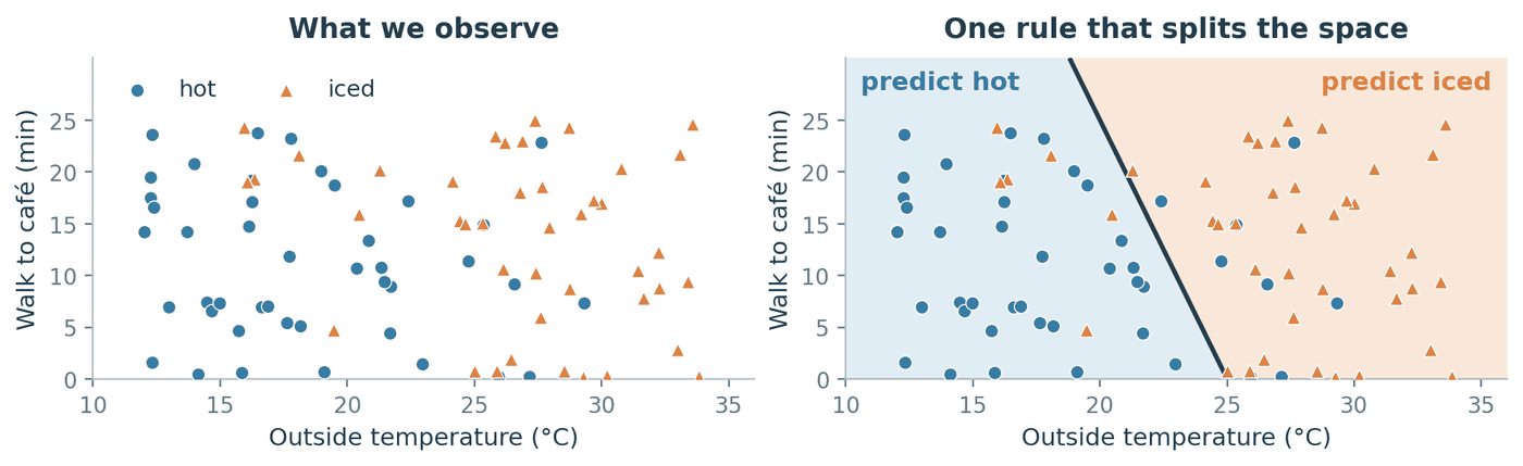
Figure 1. The same 85 orders, shown twice. On the right, every point of the plane has been coloured with the label the rule would assign it, which is what makes the rule a classifier rather than a lookup table. Customers do not all choose alike on the same day, so the two classes overlap.
Notation
| Symbol | Meaning |
|---|---|
| $n$ | number of training observations |
| $d$ | number of features (input dimensions) |
| $\mathcal{D} = \lbrace(x_i, y_i)\rbrace_{i=1}^{n}$ | the training set |
| $x_i \in \mathbb{R}^d$ | observation $i$, a vector of $d$ real numbers |
| $x_{ij}$ | feature $j$ of observation $i$ |
| $x = (x_1, \dots, x_d)^{\top}$ | a new input we have to label; $\top$ means transpose |
| $y_i \in \lbrace 0, 1\rbrace$ | the observed class of $x_i$ |
| $\hat y = f(x)$ | the label the classifier $f$ assigns to $x$ |
A classifier is therefore a function $f : \mathbb{R}^d \to \lbrace 0,1\rbrace$, and specifying $f$ is the same as specifying which region of $\mathbb{R}^d$ gets which label.
The decision boundary is the set of inputs where the predicted label changes as you cross it. With $d$ features it is normally a $(d-1)$-dimensional surface: a point on a line when $d = 1$, a curve in the plane when $d = 2$, a sheet when $d = 3$. It does not have to be connected, so a classifier can own several separate regions of the same class.
The shape of that boundary is not something we discover in the data. It is fixed in advance by the family of classifier we chose. A decision tree can only make axis-aligned steps, because each of its questions compares one feature against one threshold. KNN produces a jagged boundary assembled from straight segments, for reasons we derive in Section 2.3. Plain logistic regression produces exactly one straight cut. Hand all three the same 85 points and you get three different pictures.
Where students trip: “a good boundary gets every training point right.” Several iced orders in Figure 1 sit on the hot side, and that is not a mistake to fix. The classes genuinely overlap, because somebody does order iced coffee in November. When two classes overlap, no classifier can be right everywhere, and the lowest error rate any classifier could ever reach is called the Bayes error. It is strictly positive whenever the classes overlap. A boundary contorted enough to capture all 85 training points has stopped describing the café and started describing the noise.
2. $k$-nearest neighbours
2.1 The rule
Pick a distance function $D(x,z)$, which returns a non-negative number measuring how far apart two inputs are, and a neighbourhood size $k$, a whole number between $1$ and $n$. To label a new input $x$: find the $k$ training points closest to it under $D$, and let them vote.
Nothing is estimated and nothing is optimised. “Training” a KNN classifier means storing the training set, which is why it is often called lazy learning.
The KNN rule. Let $I_k(x)$ be the set of indices of the $k$ training points closest to $x$. Define
\[\hat p_k(x) = \frac{1}{k}\sum_{i \in I_k(x)} y_i, \qquad f_k(x) = \mathbf{1}\lbrace \hat p_k(x) \ge \tfrac{1}{2}\rbrace,\]where $\mathbf{1}\lbrace A\rbrace$ is the indicator function, equal to $1$ when the statement $A$ is true and $0$ otherwise. Since every $y_i$ is $0$ or $1$, the sum counts how many neighbours belong to class $1$, so $\hat p_k(x)$ is the fraction of the $k$ neighbours voting for class $1$. Taking $f_k = 1$ when that fraction is at least one half is exactly a majority vote, with an exact tie awarded to class $1$.
The lecture slides write the same rule with labels in $\lbrace -1, +1\rbrace$ rather than $\lbrace 0,1\rbrace$. The two forms agree, and it is worth seeing why rather than taking it on faith. Put $\tilde y_i = 2y_i - 1$, which sends $0 \mapsto -1$ and $1 \mapsto +1$. Then
\[\sum_{i \in I_k(x)} \tilde y_i = \sum_{i \in I_k(x)} (2y_i - 1) = 2\sum_{i \in I_k(x)} y_i \; - \; k = 2k\,\hat p_k(x) - k = k\left(2\hat p_k(x) - 1\right).\]The first step just expands the definition, the second splits the sum, the third substitutes $\sum_{i \in I_k(x)} y_i = k\,\hat p_k(x)$ from the definition of $\hat p_k$. Since $k > 0$, the sign of the result is the sign of $2\hat p_k(x) - 1$, which is non-negative exactly when $\hat p_k(x) \ge \frac{1}{2}$. So
\[\tilde f_k(x) = \mathrm{sign}\left(\sum_{i \in I_k(x)} \tilde y_i\right)\]is the same classifier in different clothes, as long as we set $\mathrm{sign}(0) = +1$ to match the tie convention above.
2.2 A query you can check by hand
A query sits at the origin. Five training points lie at Euclidean distances $1,\; 1.2,\; 1.5,\; 2,\; 2.2$, called $A, B, C, D, E$ in that order, with labels $1, 0, 0, 1, 1$.
| $k$ | neighbours used | votes for class 1 | $\hat p_k$ | $f_k$ |
|---|---|---|---|---|
| 1 | $A$ | 1 of 1 | $1.00$ | 1 |
| 3 | $A, B, C$ | 1 of 3 | $0.33$ | 0 |
| 5 | $A, B, C, D, E$ | 3 of 5 | $0.60$ | 1 |
The prediction goes $1 \to 0 \to 1$ on a fixed query and a fixed dataset. The only thing that moved is $k$.
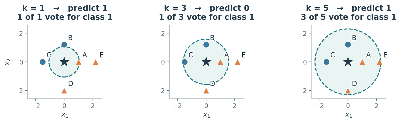
Figure 2. Widening the neighbourhood from $k=3$ to $k=5$ admits $D$ and $E$, both of class 1, which is enough to flip the answer back.
Where students trip: ties, and who breaks them. Two different ties hide here, and choosing an odd $k$ fixes only one of them.
Vote ties happen when the neighbours split evenly, for instance 2 against 2 when $k = 4$. An odd $k$ rules these out for two classes, though not for three or more.
Distance ties happen when two training points sit at exactly the same distance from the query, so “the $k$ nearest” is not well defined. An odd $k$ does nothing about this. The rule itself does not say who wins, so the answer comes down to an implementation detail of the search, and reordering the rows of your data can change a prediction.
Conventions also differ between implementations. Our rule $\mathbf{1}\lbrace \hat p_k \ge \frac{1}{2}\rbrace$ sends a vote tie to class $1$, whereas scikit-learn’s
KNeighborsClassifiertakes anargmaxover the class counts and so awards ties to the smallest class label, which is class $0$. Same data, same $k$, opposite answer.
Where students trip: “surely the closest neighbour counts for more.” Not in the rule above. Each of the $k$ selected neighbours contributes exactly one vote, so a point sitting almost on top of the query and a point barely inside the circle have identical say. Distance-weighted KNN, which gives closer neighbours larger weights, is a real and useful variant, but it is a different classifier from the one defined here.
2.3 Where the boundary comes from
Take $k = 1$ for a moment. The region of the input space that is closer to training point $x_i$ than to any other training point is called the Voronoi cell of $x_i$. Inside one cell the nearest neighbour never changes, so the prediction never changes either. The decision boundary is therefore assembled out of cell walls, and only the walls separating cells with different labels are visible in the prediction. A wall between two cells that happen to share a label is invisible: crossing it changes which point is nearest but not what that point says.
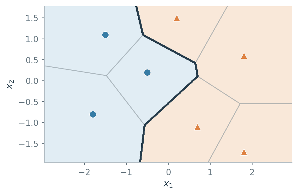
Figure 3. Thin grey lines separate Voronoi cells; the thick dark line is the decision boundary. It runs along grey lines, but only along those that separate a blue cell from an orange one.
Those walls are always flat, and the algebra shows why. For two distinct points $a$ and $b$, the wall between them is the set of $x$ equidistant from both:
\[\lVert x - a\rVert_2^2 = \lVert x - b\rVert_2^2,\]where $\lVert u\rVert_2^2 = \sum_{j=1}^{d} u_j^2$ is the squared Euclidean length of $u$. Expanding both sides with $\lVert x - a\rVert_2^2 = x^{\top}x - 2a^{\top}x + \lVert a\rVert_2^2$ gives
\[x^{\top}x - 2a^{\top}x + \lVert a\rVert_2^2 = x^{\top}x - 2b^{\top}x + \lVert b\rVert_2^2 .\]The $x^{\top}x$ term is identical on both sides and cancels. That cancellation is the whole point: it removes every quadratic term in $x$, leaving
\[2(b - a)^{\top} x = \lVert b\rVert_2^2 - \lVert a\rVert_2^2 ,\]which is a linear equation in $x$. Its solution set is the perpendicular bisector of $a$ and $b$: a line when $d = 2$, and in general a hyperplane, meaning a flat $(d-1)$-dimensional surface of the form $\lbrace x : c^{\top}x = e\rbrace$ for some fixed vector $c$ and number $e$.
Key idea. Every individual piece of a 1-NN boundary is flat, yet the boundary as a whole curves, because it is stitched together from many such pieces. KNN is nonparametric, meaning the model has no fixed-size parameter vector and what it stores grows with $n$. That is what lets it trace a shape you never had to specify in advance.
3. Choosing $k$
3.1 Why training error cannot do it
The obvious quantity to minimise is the training error, the fraction of training points the classifier gets wrong:
\[\hat R_n(f_k) = \frac{1}{n}\sum_{i=1}^{n} \mathbf{1}\lbrace f_k(x_i) \ne y_i\rbrace.\]It is the wrong tool here, and it fails in a way worth understanding rather than memorising.
Where students trip: “pick the $k$ with the lowest training error.” Evaluate $f_1$ at a training point $x_i$. Its nearest neighbour is itself, at distance $0$, so the vote returns $y_i$ and the prediction is right. Repeat for every $i$. As long as the inputs are distinct and a point is allowed to be its own neighbour, $\hat R_n(f_1) = 0$ always, even if you shuffled every label first. Training error does not rank the candidate values of $k$; it crowns $k = 1$ every time.
Two caveats. If two identical inputs carry conflicting labels, one of them must be wrong and the error is no longer zero. And leave-one-out evaluation removes the shortcut by construction, since it forbids a point from being its own neighbour.
So we need data the model has not memorised, which is what a validation set is for: a slice of labelled data held out of training, used only to compare candidate models.
What $k$ is really trading. Small $k$ gives high variance: one or two observations decide the prediction at a point, so redrawing the sample redraws the boundary. Large $k$ gives high bias: the neighbourhood keeps growing until it reaches across a real class boundary and averages the two classes together, which smooths away structure that was genuinely there. At the extreme $k = n$ every query uses all $n$ training points, so every input receives the training set’s majority label and the classifier is a constant.
3.2 An experiment
The dataset is 360 points in two interleaved arcs. The split into 216 training, 72 validation and 72 test points was fixed before anything was measured, and the features were standardised using training statistics only, for reasons covered in Section 4.2.
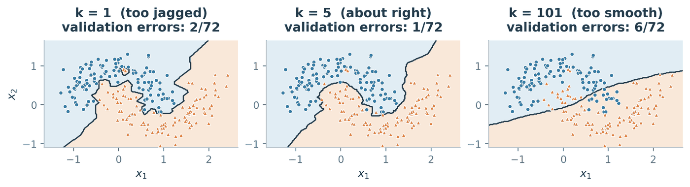
Figure 4. At $k=1$ a single oddly placed label carves out its own island. At $k=101$ the neighbourhood is wide enough to average the two arcs into a nearly straight cut, which no longer follows the shape of either one.
Sweeping $k$ over the odd numbers from 1 to 101 gives the two curves below. Odd values avoid vote ties.
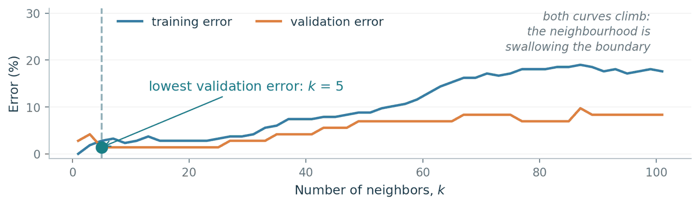
Figure 5. Training and validation error against $k$. Note the left edge: training error is $0\%$ at $k=1$ by construction, which is precisely why the blue curve cannot be used to choose anything.
The lowest validation error is $1/72$, reached at $k = 5$; when several values tie, the convention is to take the smallest, since it is the least smoothed model consistent with the evidence. That model makes $6/216$ training errors and $4/72$ test errors, so the honest final accuracy is $68/72 = 94.4\%$.
ks   = np.arange(1, 102, 2)                              # odd k only
err  = [np.sum(predict(Z[va], k) != y[va]) for k in ks]  # validation errors
best = ks[np.argmin(err)]                                # chosen here...
print(best, np.sum(predict(Z[te], best) != y[te]))       # ...scored here
# 5 4
Where students trip: “validation error estimates test error.” Above, validation error came out at $1/72 = 1.4\%$ but test error at $4/72 = 5.6\%$. The supposedly pessimistic number was the smaller one, and this is the normal direction of the bias rather than bad luck. We tried 51 candidate values of $k$ and kept whichever scored best on the validation set, so part of that winning score reflects the model being good and part reflects us having searched. Once a set of data has been used to make a choice, it can no longer give an unbiased measurement of that choice. This is the entire reason for keeping a third, untouched split.
Key idea. Choose $k$ on validation data or by cross-validation, then report that one chosen model’s error on test data you have never looked at. A larger $k$ is not inherently safer. It is a different point on the bias/variance trade, and only the data can say which point is right.
4. Distance, units, and scaling
Every result so far assumed some $D(x,z)$ without saying which. That choice is not a detail.
4.1 The metric itself changes the answer
The two usual choices are
\[D_2(x,z) = \sqrt{\sum_{j=1}^{d}(x_j - z_j)^2}, \qquad D_1(x,z) = \sum_{j=1}^{d} \lvert x_j - z_j \rvert,\]called the Euclidean (or $L_2$) and Manhattan (or $L_1$) distances. The second is named after walking along a street grid, since it adds up the moves along each axis separately instead of cutting across.
Worked example. Query at the origin. Take $a = (2,2)$ labelled $0$ and $b = (3,0)$ labelled $1$.
Euclidean: $D_2(0,a) = \sqrt{4+4} = \sqrt{8} \approx 2.83$ and $D_2(0,b) = \sqrt{9+0} = 3$. Since $2.83 < 3$, the nearest neighbour is $a$ and 1-NN predicts $0$.
Manhattan: $D_1(0,a) = 2 + 2 = 4$ and $D_1(0,b) = 3 + 0 = 3$. Since $4 > 3$, the nearest neighbour is $b$ and 1-NN predicts $1$.
Same points, same labels, same $k$, opposite prediction.
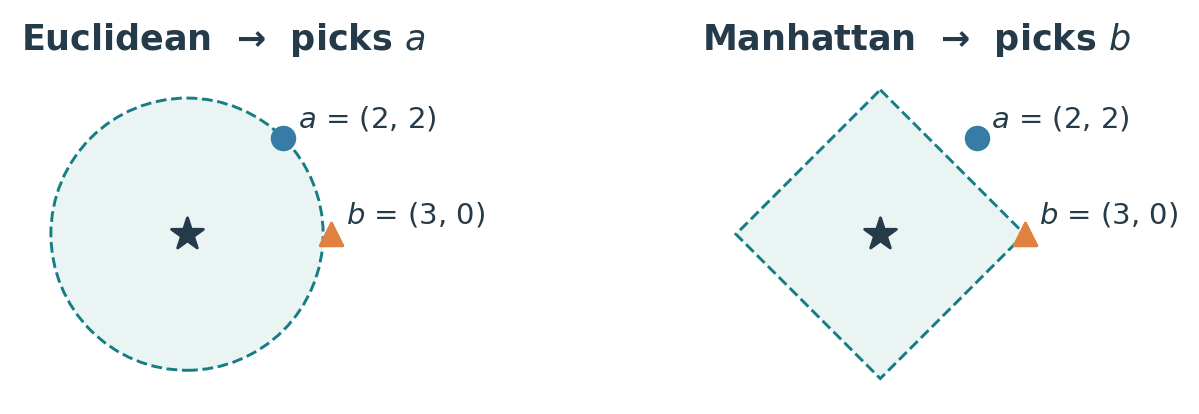
Figure 6. The shaded region holds every point within the nearest-neighbour distance of the query. The Euclidean ball is round and reaches the diagonal point first; the Manhattan ball is a diamond and reaches the on-axis point first.
4.2 Units change the answer too
Choosing a metric is at least a deliberate act. The next failure is not.
Worked example. A new order sits at $q = (24^{\circ}\mathrm{C},\; 10\ \text{min})$. Two past orders are $A = (25^{\circ}\mathrm{C},\; 13\ \text{min})$, hot, and $B = (29^{\circ}\mathrm{C},\; 10.2\ \text{min})$, iced.
units $D_2(q, A)$ $D_2(q, B)$ nearest 1-NN says minutes $\sqrt{1^2 + 3^2} = 3.16$ $\sqrt{5^2 + 0.2^2} = 5.00$ $A$ hot seconds $\sqrt{1^2 + 180^2} = 180.00$ $\sqrt{5^2 + 12^2} = 13.00$ $B$ iced standardised $\sqrt{0.2^2 + 0.3^2} = 0.36$ $\sqrt{1^2 + 0.02^2} = 1.00$ $A$ hot Row two describes the same café, the same customers and the same arithmetic as row one. We multiplied one column by 60 and the prediction changed.
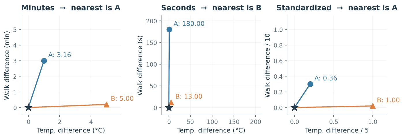
Figure 7. In minutes, the 3-minute gap to $A$ and the 5-degree gap to $B$ are comparable quantities. In seconds that same gap becomes 180 and swamps temperature completely, so the distance is now measuring walking time and almost nothing else.
The fix is to put every feature on a common footing before measuring anything. The usual choice is standardisation:
\[x'_{ij} = \frac{x_{ij} - \mu_j}{s_j},\]where $\mu_j$ and $s_j$ are the mean and standard deviation of feature $j$ computed over the training set.
This genuinely removes the dependence on units, and the reason is short enough to verify. Suppose we re-express feature $j$ in a unit that is $c$ times smaller, so every value becomes $c\,x_{ij}$ (minutes to seconds is $c = 60$). The mean scales the same way, $\mu_j \mapsto c\,\mu_j$, and so does the standard deviation, $s_j \mapsto c\,s_j$, because both are measured in the units of the feature. The standardised value is then
\[\frac{c\,x_{ij} - c\,\mu_j}{c\,s_j} = \frac{c\,(x_{ij} - \mu_j)}{c\,s_j} = \frac{x_{ij} - \mu_j}{s_j},\]which is exactly what it was before. The factor $c$ cancels, so every standardised distance, and therefore every neighbour list and every prediction, is unchanged. In the table above, the walking-time divisor of $10$ minutes would become $600$ seconds and reproduce the same $0.36$ and $1.00$.
Where students trip: fitting the scaler on the wrong rows. Compute $\mu_j$ and $s_j$ from the training rows only, then apply those same numbers to validation and test. If you standardise the whole dataset first, the test set has influenced the transformation applied to the training set, and your reported error stops being an estimate of performance on unseen data. Inside cross-validation this means re-fitting the scaler separately in every fold. Two smaller points: a constant feature has $s_j = 0$, so guard the division; and standardising an irrelevant feature does not make it harmless, it just guarantees it an equal say.
4.3 Why this gets worse in high dimensions
Distance also becomes less informative as $d$ grows. Draw 1000 points uniformly at random in the unit cube $[0,1]^d$ and, from one of them, take the ratio of the farthest distance to the nearest:
| dimension $d$ | 2 | 5 | 10 | 50 | 200 | 1000 |
|---|---|---|---|---|---|---|
| farthest / nearest | 98.5 | 9.4 | 3.8 | 1.66 | 1.28 | 1.12 |
In two dimensions the nearest point is about a hundred times closer than the farthest, so the word “nearest” is picking out something meaningful. By $d = 1000$ the farthest of a thousand points is only $12\%$ farther away than the nearest. Every point is roughly equidistant from every other, and the neighbour list stops carrying information about which points are genuinely similar.
The mechanism is easy to see. The squared Euclidean distance between two points is a sum of $d$ per-coordinate contributions, one from each feature. Adding more independent contributions makes the total grow steadily, but the fluctuations partly cancel, so the typical distance grows while the spread of distances barely moves. Measuring this on random pairs in $[0,1]^d$:
| dimension $d$ | 2 | 10 | 100 | 1000 |
|---|---|---|---|---|
| mean distance | 0.52 | 1.27 | 4.08 | 12.91 |
| standard deviation of distance | 0.25 | 0.25 | 0.24 | 0.24 |
The mean grows roughly like $\sqrt{d}$ while the standard deviation stays near $0.25$, so the distances bunch ever more tightly around a common value. Since KNN only ever uses the ordering of distances, and that ordering is decided by differences that are shrinking relative to the distances themselves, the neighbour list becomes increasingly arbitrary. Irrelevant features make this worse directly: each one contributes to the distance without contributing any information about the label.
5. What KNN buys you, and what it costs
The whole trade in one place:
| Strengths | Limitations | |
|---|---|---|
| Fitting | No training phase at all. Adding data means appending rows. | Nothing is ever summarised, so there is no compact model to inspect or ship. |
| Flexibility | Nonparametric, so it traces curved and disconnected boundaries with no shape specified in advance (Figure 3, Figure 4). | The same flexibility means small $k$ chases label noise (Section 7). |
| Interpretability | A prediction is justified by naming actual training examples. | Choosing $k$ needs held-out data; training error is useless (Section 3.1). |
| Assumptions | Only that “close inputs tend to share labels” under your $D$. | It inherits every flaw in $D$: metric choice, feature units, irrelevant features, high $d$ (Section 4). |
| Cost | Memory and time are trivial for small $n$. | Both memory and per-prediction time grow with $n$, which is the bottleneck below. |
Inference cost
| KNN | a fitted linear score | |
|---|---|---|
| what is stored | $n$ vectors of $d$ features, plus $n$ labels | $d$ weights and one intercept |
| memory | $O(nd)$ | $O(d)$ |
| cost of training | none | one optimisation, paid once |
| cost per prediction | $O(nd)$ | $O(d)$ |
The notation $O(\cdot)$ describes how a cost grows with the inputs, ignoring constant factors. Both KNN entries are worth deriving rather than quoting.
Memory. Storing $n$ observations of $d$ numbers each means storing $nd$ numbers, hence $O(nd)$. The labels add $n$ more, which is smaller than $nd$ and so does not change the order.
Prediction. To find the neighbours of one query $x$, you must know its distance to every training point, because a point you never measured could always have been the closest. Each distance $D_2(x, x_i)$ touches all $d$ coordinates, costing $O(d)$. Doing that $n$ times costs $O(nd)$. Picking the $k$ smallest of those $n$ distances costs a further $O(n)$ using linear-time selection, giving a total of $O(nd + n) = O(nd)$ for $d \ge 1$. If you sort the whole list instead, the total is $O(nd + n \log n)$; the sorting term can dominate when $d$ is small.
Put numbers on it. At $n = 10^{6}$ and $d = 100$, a single prediction touches $10^{8}$ feature coordinates, and the entire training set has to be deployed wherever predictions are made. A café app would be shipping every order it has ever taken, and repeating that work per customer.
Spatial index structures help. A KD-tree or a ball tree costs about $O(n \log n)$ to build and can bring a query close to $O(\log n)$ by ruling out whole groups of points without measuring them individually. That is a best case in low dimensions rather than a guarantee, and by Section 4.3 high $d$ is exactly where the pruning stops working, because no group of points is far enough away to rule out.
Key idea, and the reason we move on. KNN pays nothing to train and pays per prediction, with a bill that grows with the dataset. A parametric model inverts this: it has a fixed-size parameter vector, fits it once up front, and then predicts in $O(d)$ using a model whose size does not depend on $n$ at all. It also throws away the raw data, which is a cost in flexibility and a benefit in storage. That inversion, rather than accuracy, is what motivates the rest of the lecture.
6. Logistic regression
6.1 From odds to the sigmoid
We want to model
\[p(x) = P(Y = 1 \mid X = x)\]directly, as a function of $x$ with a fixed number of coefficients. Here $X$ is the random feature vector and $Y$ the random label, so $p(x)$ is the probability that an input with features $x$ belongs to class $1$.
The obstacle is a range mismatch. A probability must lie in $[0,1]$, while a linear function $b + w^{\top}x$ can take any real value, so we cannot simply set the two equal and fit.
The standard escape is to model the odds instead of the probability. The odds of class $1$ are $p/(1-p)$: if $p = 0.8$ then the odds are $0.8/0.2 = 4$, read as “4 to 1”. As $p$ ranges over $(0,1)$, the numerator is positive and the denominator is positive, so the odds are always positive; and as $p \to 1$ the denominator goes to $0$ and the odds grow without bound. The odds therefore cover $(0, \infty)$. Taking the natural logarithm of a quantity on $(0,\infty)$ produces a value on $(-\infty, \infty)$, which is precisely the range a linear function can produce. The mismatch is gone.
The logistic regression model.
\[\log \frac{p(x)}{1 - p(x)} = b + w^{\top} x = s(x),\]with weight vector $w \in \mathbb{R}^d$, intercept $b \in \mathbb{R}$, natural logarithm, and $s(x)$ called the score. The left-hand side is the log-odds, sometimes called the logit. To absorb the intercept into the dot product, write $\bar x = (1, x^{\top})^{\top}$ and $\bar w = (b, w^{\top})^{\top}$, so that $s(x) = \bar w^{\top}\bar x$.
Solving for $p$ takes three steps, and it is worth doing once by hand. Write $s$ for $s(x)$ and $p$ for $p(x)$. Exponentiating both sides removes the logarithm:
\[\frac{p}{1-p} = e^{s} \;\Longrightarrow\; p = e^{s}(1-p) = e^{s} - e^{s}p \;\Longrightarrow\; p + e^{s}p = e^{s} \;\Longrightarrow\; p\,(1 + e^{s}) = e^{s}.\]Dividing by $1 + e^{s}$, which is never zero, and then dividing numerator and denominator by $e^{s}$:
\[p(x) = \sigma\left(s(x)\right), \qquad \sigma(s) = \frac{e^{s}}{1 + e^{s}} = \frac{1}{1 + e^{-s}},\]where $\sigma$ is the sigmoid (or logistic) function.
Where students trip: the name. Logistic regression is a classifier. The word “regression” survives because we are fitting a linear model, but we are fitting it to the log-odds rather than to the label. Nobody is predicting a continuous $y$.
The café model we will work with is $s(T, M) = 0.30\,T + 0.06\,M - 7.5$, with $T$ the temperature in degrees Celsius and $M$ the walking time in minutes.
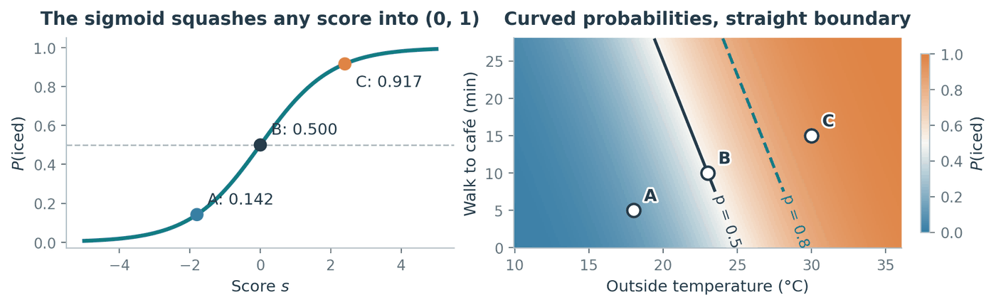
Figure 8. The colour on the right varies smoothly across the plane, yet the solid $p = 0.5$ contour, which is the decision boundary, is perfectly straight. Section 6.2 explains why those two facts are compatible.
6.2 Two facts about the sigmoid
The derivative has a tidy closed form. With $\sigma(s) = (1 + e^{-s})^{-1}$, the chain rule gives
\[\sigma'(s) = -(1 + e^{-s})^{-2} \cdot \frac{d}{ds}\left(1 + e^{-s}\right) = -(1+e^{-s})^{-2} \cdot (-e^{-s}) = \frac{e^{-s}}{(1 + e^{-s})^{2}}.\]Now split that single fraction into a product of two:
\[\sigma'(s) = \frac{1}{1 + e^{-s}} \cdot \frac{e^{-s}}{1 + e^{-s}} = \sigma(s)\left(1 - \sigma(s)\right).\]The first factor is $\sigma(s)$ by definition. The second is $1 - \sigma(s)$, because
\[1 - \frac{1}{1+e^{-s}} = \frac{(1 + e^{-s}) - 1}{1 + e^{-s}} = \frac{e^{-s}}{1+e^{-s}}.\]Two consequences follow. Since $\sigma$ takes values strictly between $0$ and $1$, the product $\sigma(1-\sigma)$ is strictly positive, so $\sigma$ is strictly increasing everywhere. And it is largest when $\sigma = \frac{1}{2}$, giving a maximum slope of $\frac{1}{4}$ at $s = 0$. This identity reappears the moment we differentiate the log-likelihood to actually fit $w$.
Thresholding the probability is thresholding the score. Setting $s = 0$ gives $\sigma(0) = 1/(1 + e^{0}) = 1/2$. Because $\sigma$ is strictly increasing, $\sigma(s) \ge \frac{1}{2}$ happens exactly when $s \ge 0$. Therefore
\[p(x) \ge \tfrac{1}{2} \iff s(x) \ge 0 \iff b + w^{\top}x \ge 0 .\]Key idea. The probability surface is curved, but the decision boundary $\lbrace x : b + w^{\top}x = 0\rbrace$ is a flat hyperplane whenever $w \ne 0$. Applying a strictly increasing function to a score cannot change which side of a threshold anything lands on, so all the curvature of $\sigma$ happens along the score axis and none of it reaches the boundary.
6.3 A worked prediction
Each prediction is three steps: $(T,M) \to s \to p = \sigma(s) \to \hat y = \mathbf{1}\lbrace p \ge \frac{1}{2}\rbrace$.
| order | $T$ | $M$ | score $s = 0.30T + 0.06M - 7.5$ | $p = \sigma(s)$ | $\hat y$ |
|---|---|---|---|---|---|
| $A$ | 18 | 5 | $5.4 + 0.3 - 7.5 = -1.8$ | $0.142$ | hot |
| $B$ | 23 | 10 | $6.9 + 0.6 - 7.5 = 0$ | $0.500$ | iced (by the tie rule) |
| $C$ | 30 | 15 | $9.0 + 0.9 - 7.5 = 2.4$ | $0.917$ | iced |
For $A$: $\sigma(-1.8) = 1/(1 + e^{1.8}) = 1/(1 + 6.050) = 0.142$.
6.4 Moving the threshold
Nothing forces the cutoff to be $\frac{1}{2}$. That particular choice says a false hot and a false iced cost the same, which is a claim about the café, not about the model. For a general threshold $\tau \in (0,1)$, the same monotonicity argument gives
\[p(x) \ge \tau \iff \frac{p(x)}{1 - p(x)} \ge \frac{\tau}{1 - \tau} \iff b + w^{\top}x \ge \log\frac{\tau}{1-\tau},\]where the first step holds because $p \mapsto p/(1-p)$ is increasing on $(0,1)$, and the second because $\log$ is increasing and the left side is the log-odds, which equals $b + w^{\top}x$ by definition.
The right-hand side is a constant, so raising $\tau$ shifts the boundary without rotating it: the vector $w$, which sets the boundary’s orientation, does not appear. Requiring $\tau = 0.8$ means requiring $s \ge \log 4 \approx 1.386$. For a fixed 10-minute walk, the temperature cutoff moves from $23^{\circ}\mathrm{C}$ to
\[T = \frac{7.5 + \log 4 - 0.06(10)}{0.30} = \frac{7.5 + 1.386 - 0.6}{0.30} \approx 27.62^{\circ}\mathrm{C}.\]Order $B$ is now predicted hot, while $C$ stays iced. Notice what did not change: $B$’s probability is still exactly $0.500$. We changed how much evidence we demand before acting, not what the model believes.
6.5 The same boundary can carry very different confidence
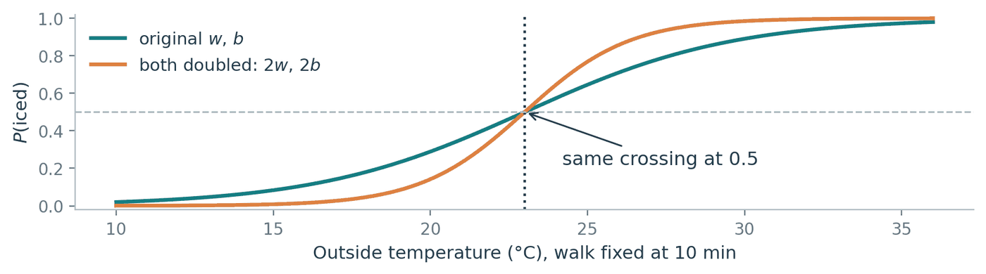
Figure 9. Doubling the coefficients leaves the crossing at $p = 0.5$ exactly where it was, so both models predict identically on every input. The orange curve is simply far more emphatic about it.
Replacing $(w, b)$ by $(2w, 2b)$ maps $s \mapsto 2s$. The set where $s = 0$ is unchanged, because $2s = 0$ exactly when $s = 0$, so not one prediction differs. Yet at order $C$ the reported probability climbs from $\sigma(2.4) = 0.917$ to $\sigma(4.8) = 0.992$.
Where students trip: reading confidence off a boundary plot. Two models with pixel-identical decision boundaries can report very different probabilities, and a boundary picture cannot tell them apart. If you care about the $0.9$ in “90% confident”, which you do for ranking, for choosing a threshold, or for computing an expected cost, you have to check calibration separately. A predicted probability is an estimate produced by a model you assumed, not a measured frequency.
Where students trip: what the coefficients mean. Raising the temperature by $1^{\circ}\mathrm{C}$ adds $0.30$ to the log-odds, which multiplies the odds by $e^{0.30} \approx 1.35$. It does not add a fixed amount to the probability. From $18^{\circ}$ to $19^{\circ}$ the probability moves $0.142 \to 0.182$, a jump of $0.041$; from $30^{\circ}$ to $31^{\circ}$ the same coefficient moves it $0.917 \to 0.937$, a jump of only $0.020$. The odds scale by a constant factor, the probability does not.
Where students trip: “logistic regression can only draw straight lines.” It draws a hyperplane in whatever features you hand it. Feed it $(x_1, x_2, x_1^2, x_2^2, x_1x_2)$ and the boundary $b + w^{\top}x = 0$ becomes a conic section back in the original plane, since that equation is now quadratic in $x_1$ and $x_2$. The model is linear in $w$, not in your raw measurements. So the two interleaved arcs of Section 3 are out of reach for logistic regression on $(x_1, x_2)$ alone, and well within reach once the right features are added.
6.6 Discriminative, not generative
Logistic regression models $P(Y \mid X)$ and never models $P(X)$. Models of this kind are called discriminative; models that instead describe how the data were generated, by modelling $P(X \mid Y)$ and $P(Y)$, are called generative.
Skipping $P(X)$ is the point rather than an oversight. Estimating a probability density in $d$ dimensions is hard and needs a lot of data, and you do not need one in order to draw a boundary, so a discriminative model spends its capacity on the question actually being asked. This is also the usual explanation for why such models tend to classify well in practice. The price is that the model cannot generate new feature vectors, because it never learned what a plausible input looks like.
7. A small experiment: what one wrong label costs
To make the bias/variance story concrete, here is one experiment small enough to check entirely by hand.
The true rule is $y = \mathbf{1}\lbrace x > 0.5\rbrace$ in one dimension. Training inputs sit at the integers $-5, -4, \dots, 5$. Testing uses 2000 evenly spaced points across $[-5, 5]$, placed at midpoints so that no test point is ever exactly tied between two training inputs. Three runs: clean labels, one flipped label at $x = -3$, and two adjacent flips at $x = -3$ and $x = -2$.
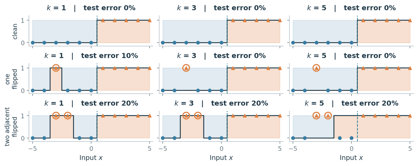
Figure 10. Circled markers are the corrupted labels. The shaded step function is the prediction; the dashed line is the true boundary at $0.5$.
| training labels | $k=1$ | $k=3$ | $k=5$ |
|---|---|---|---|
| clean | $0\%$ | $0\%$ | $0\%$ |
| one flipped at $-3$ | $10\%$ | $0\%$ | $0\%$ |
| two flipped at $-3, -2$ | $20\%$ | $20\%$ | $20\%$ |
Each entry can be worked out exactly, and doing so is more useful than reading the percentages off the plot.
One flipped label, $k = 1$. A test point $q$ has $x = -3$ as its nearest training input exactly when $q$ lies between the midpoint of $-4$ and $-3$ and the midpoint of $-3$ and $-2$, that is on $(-3.5, -2.5)$. Throughout that interval 1-NN returns the corrupted label $1$ while the truth is $0$. The interval has length $1$ inside a test range of length $10$, so the error is $10\%$.
One flipped label, $k = 3$. For any $q$ in $(-3.5, -2.5)$, the three nearest training inputs are $-4$, $-3$ and $-2$, whose labels are $0$, $1$, $0$. The majority is $0$, which is correct, and the corrupted point is outvoted two to one. Outside that interval, $-3$ can still be among the three nearest inputs: near $q = -4$, for example, they are $-4$, $-5$ and $-3$. Whenever $-3$ is included, the other two neighbours have label $0$ and outvote it; when it is absent, the prediction is unchanged from the clean-label case. The error is $0\%$, and the same argument works for $k = 5$.
Two adjacent flips, $k = 3$. Now the labels at $-3$ and $-2$ are both $1$. For $q$ just left of $-3$ the three nearest inputs are $-3, -4, -2$ with labels $1, 0, 1$, so the majority is $1$ and wrong. For $q$ just right of $-2$ the three nearest are $-2, -1, -3$ with labels $1, 0, 1$, again wrong. Working out where the prediction flips back gives a wrong region of $(-3.5, -1.5)$, length $2$, so $20\%$. Averaging did not help, because the two mistakes back each other up.
Two adjacent flips, $k = 5$. Something slightly different happens. Near $-3$ the five nearest inputs are $-3, -4, -2, -5, -1$ with labels $1, 0, 1, 0, 0$, giving $\hat p_5 = 2/5 < 1/2$ and the correct answer $0$. The wider window has diluted the two bad votes. But at $q = -1.4$ the five nearest are $-1, -2, 0, -3, 1$ with labels $0, 1, 0, 1, 1$, giving $\hat p_5 = 3/5 \ge 1/2$ and the wrong answer $1$. The prediction switches to $1$ at $q = -1.5$ and stays there, so the wrong region is $(-1.5, 0.5)$, again length $2$ and $20\%$. The damage did not shrink; it slid across and parked itself against the true boundary.
x     = np.arange(-5.0, 6.0)                       # training inputs
q     = -5 + (np.arange(2000) + 0.5) * 10 / 2000   # midpoints: no distance ties
truth = (q > 0.5).astype(int)
order = np.argsort(abs(q[:, None] - x), axis=1, kind="stable")

for flips in ([], [-3], [-3, -2]):
    y = (x > 0.5).astype(int)
    for location in flips:
        y[x == location] = 1 - y[x == location]
    errors = [round(100 * np.mean(
                  (y[order[:, :k]].mean(1) >= 0.5).astype(int) != truth))
              for k in (1, 3, 5)]
    print(flips, errors)
# []        [0, 0, 0]
# [-3]      [10, 0, 0]
# [-3, -2]  [20, 20, 20]
Key idea. Averaging over neighbours repairs isolated label mistakes and is helpless against correlated ones, because a large enough $k$ dilutes one bad vote but a cluster of bad votes simply moves the majority with it. And the punchline: 1-NN’s training error is $0\%$ in all three runs, while its test error is $0\%$, $10\%$ and $20\%$. Reproducing every recorded label perfectly is not evidence that anything was learned.
Summary
- A classifier partitions the input space, and the decision boundary is where that partition changes. Its shape is chosen by the model family, not discovered in the data.
- KNN stores the training set and takes a majority vote among the $k$ nearest points. Its boundary is built from perpendicular bisectors, so it is flat in pieces and curved overall.
- Training error cannot select $k$, because 1-NN scores a perfect $0$ by construction. Select on validation data, then report on a test set you have not touched.
- Small $k$ means high variance, large $k$ means high bias. Neither extreme is safe, and larger is not automatically better.
- KNN is only as good as its distance function, which makes it only as good as your feature units, your feature choices and your dimension count.
- KNN costs nothing to fit and $O(nd)$ per prediction. A parametric model inverts that, which is why we move to one.
- Logistic regression makes the log-odds linear in $x$. The probability therefore curves through $\sigma$ while the boundary stays a hyperplane, and each prediction costs $O(d)$ instead of $O(nd)$.
Notation reference
| Symbol | Meaning | Introduced |
|---|---|---|
| $n$, $d$ | number of training points, number of features | §1 |
| $\mathcal{D}$, $x_i$, $x_{ij}$, $y_i$ | training set, observation, one feature of it, its label | §1 |
| $x$, $\hat y$, $f$ | a new input, its predicted label, the classifier | §1 |
| $\mathbf{1}\lbrace A\rbrace$ | indicator: $1$ if $A$ is true, else $0$ | §2.1 |
| $D(x,z)$, $D_1$, $D_2$ | a distance function; Manhattan and Euclidean | §2.1, §4.1 |
| $k$, $I_k(x)$ | neighbourhood size, indices of the $k$ nearest points | §2.1 |
| $\hat p_k(x)$, $f_k(x)$ | fraction of neighbours voting class 1, the KNN prediction | §2.1 |
| $\tilde y_i$, $\mathrm{sign}$ | labels rescaled to $\lbrace -1,+1\rbrace$, the sign function | §2.1 |
| $\lVert u \rVert_2^2$ | squared Euclidean length, $\sum_j u_j^2$ | §2.3 |
| $\hat R_n(f)$ | training error of $f$ | §3.1 |
| $\mu_j$, $s_j$, \(x'_{ij}\) | training mean, training standard deviation, standardised value | §4.2 |
| $O(\cdot)$ | order of growth, ignoring constants | §5 |
| $X$, $Y$ | the random feature vector and random label | §6.1 |
| $p(x)$ | $P(Y = 1 \mid X = x)$ | §6.1 |
| $w$, $b$, $s(x)$ | weight vector, intercept, score $b + w^{\top}x$ | §6.1 |
| $\bar x$, $\bar w$ | input and weights with the intercept absorbed | §6.1 |
| $\sigma(s)$ | sigmoid, $1/(1 + e^{-s})$ | §6.1 |
| $\tau$ | probability threshold for deciding class 1 | §6.4 |
References
The development of $k$-nearest neighbours and logistic regression in these notes follows [1], and the scope, notation and worked ordering follow [2].
[1] M. Gönen, ENGR 421: Introduction to Machine Learning. Koç University, College of Engineering, 2024. Lecture slides and course notes.
[2] K. Wang, CSE/ISyE 6740: Computational Data Analysis, Lecture 7, “Logistic Regression and Support Vector Machine”. Georgia Institute of Technology, 16 September 2026.
English is not my first language; Claude was used to polish the wording.
Assignment pending
Develop the assigned part of the lecture’s core course materials.
The course team will assign this section through a GitHub issue.
Assignment pending
Develop an optional extension, application, or related topic assigned for this lecture.
The course team will assign this section through a GitHub issue.
Assignment pending
Develop an optional extension, application, or related topic assigned for this lecture.
The course team will assign this section through a GitHub issue.